The wflow_hbv model¶

Introduction¶

The Hydrologiska Byrans Vattenbalansavdelning (HBV) model was introduced back in 1972 by the Swedisch Meteological and Hydrological Institute (SMHI). The HBV model is mainly used for runoff simulation and hydrological forecasting. The model is particularly useful for catchments where snow fall and snow melt are dominant factors, but application of the model is by no means restricted to these type of catchments.

Description¶

The model is based on the HBV-96 model. However, the hydrological routing represent in HBV by a triangular function controlled by the MAXBAS parameter has been removed. Instead, the kinematic wave function is used to route the water downstream. All runoff that is generated in a cell in one of the HBV reservoirs is added to the kinematic wave reservoir at the end of a timestep. There is no connection between the different HBV cells within the model. Wherever possible all functions that describe the distribution of parameters within a subbasin have been removed as this is not needed in a distributed application/

A catchment is divided into a number of grid cells. For each of the cells individually, daily runoff is computed through application of the HBV-96 of the HBV model. The use of the grid cells offers the possibility to turn the HBV modelling concept, which is originally lumped, into a distributed model.

Schematic view of the relevant components of the HBV model

The figure above shows a schematic view of hydrological response simulation with the HBV-modelling concept. The land-phase of the hydrological cycle is represented by three different components: a snow routine, a soil routine and a runoff response routine. Each component is discussed separately below.

The snow routine¶

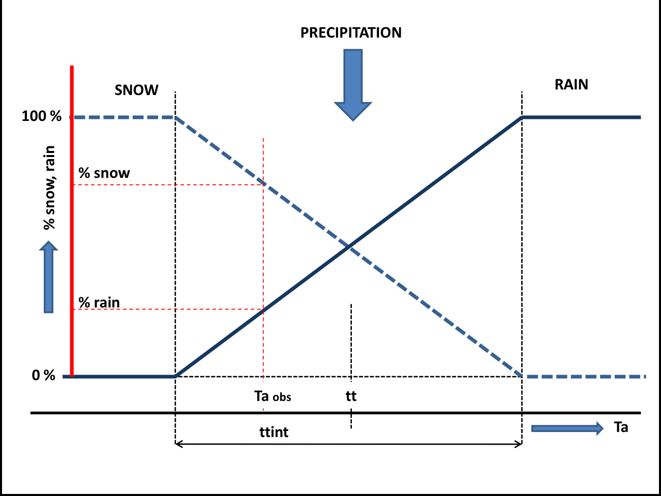
Precipitation enters the model via the snow routine. If the air temperature, $T_{a}$ , is below a user-defined threshold $TT (\approx0^{o}C)$ precipitation occurs as snowfall, whereas it occurs as rainfall if $T_{a}\geq TT$ . A another parameter $TTI$ defines how precipitation can occur partly as rain of snowfall (see the figure below). If precipitation occurs as snowfall, it is added to the dry snow component within the snow pack. Otherwise it ends up in the free water reservoir, which represents the liquid water content of the snow pack. Between the two components of the snow pack, interactions take place, either through snow melt (if temperatures are above a threshold $TT$ ) or through snow refreezing (if temperatures are below threshold $TT$ ). The respective rates of snow melt and refreezing are:

$Q_{m} = cfmax(T_{a}-TT)\;\;;T_{a}>TT Q_{r} = cfmax*cfr(TT-T_{a})\;;T_{a}<TT$

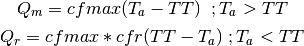
where $Q_{m}$ is the rate of snow melt, $Q_{r}$ is the rate of snow refreezing, and $cfmax$ and $cfr$ are user defined model parameters (the melting factor $mm/(^{o}C*day)$ and the refreezing factor respectively)

Note

The FoCFMAX parameter from the original HBV version is not used. instead the CFMAX is presumed to be for the landuse per pixel. Normally for forested pixels the CFMAX is 0.6 {*} CFMAX

The air temperature, $T_{a}$ , is related to measured daily average temperatures. In the original HBV-concept, elevation differences within the catchment are represented through a distribution function (i.e. a hypsographic curve) which makes the snow module semi-distributed. In the modified version that is applied here, the temperature, $T_{a}$ , is represented in a fully distributed manner, which means for each grid cell the temperature is related to the grid elevation.

The fraction of liquid water in the snow pack (free water) is at most equal to a user defined fraction, $WHC$ , of the water equivalent of the dry snow content. If the liquid water concentration exceeds $WHC$ , either through snow melt or incoming rainfall, the surpluss water becomes available for infiltration into the soil:

$Q_{in}=max\{(SW-WHC*SD);\;0.0\}$

where $Q_{in}$ is the volume of water added to the soil module, $SW$ is the free water content of the snow pack and $SD$ is the dry snow content of the snow pack.

Schematic view of the snow routine

Potential Evaporation¶

The original HBV version includes both a multiplication factor for potential evaporation and a exponential reduction factor for potential evapotranspiration during rain events. The $CEVPF$ factor is used to connect potential evapotranspiration per landuse. In the original version the $CEVPFO$ is used and it is used for forest landuse only.

Interception¶

The parameters $ICF0$ and $ICFI$ introduce interception storage for forested and non-forested zones respectively in the original model. Within our application this is replaced by a single $ICF$ parameter assuming the parameter is set for each grid cell according to the land-use. In the original application it is not clear if interception evaporation is subtracted from the potential evaporation. In this implementation we dos subtract the interception evaporation to ensure total evaporation does not exceed potential evaporation. From this storage evaporation equal to the potential rate $ET_{p}$ will occur as long as water is available, even if it is stored as snow. All water enters this store first, there is no concept of free throughfall (e.g. through gaps in the canopy). In the model a running water budget is kept of the interception store:

The available storage (ICF-Actual storage) is filled with the water coming from the snow routine ( $Q_{in}$ )

Any surplus water now becomes the new $Q_{in}$

Interception evaporation is determined as the minimum of the current interception storage and the potential evaporation

The soil routine¶

The incoming water from the snow and interception routines, $Q_{in}$ , is available for infiltration in the soil routine. The soil layer has a limited capacity, $F_{c}$ , to hold soil water, which means if $F_{c}$ is exceeded the abundant water cannot infiltrate and, consequently, becomes directly available for runoff.

$Q_{dr}=max\{(SM+Q_{in}-F_{c});\;0.0\}$

where $Q_{dr}$ is the abundant soil water (also referred to as direct runoff) and $SM$ is the soil moisture content. Consequently, the net amount of water that infiltrates into the soil, $I_{net}$ , equals:

$I_{net}=Q_{in}-Q_{dr}$

Part of the infiltrating water, $I_{net}$ , will runoff through the soil layer (seepage). This runoff volume, $SP$ , is related to the soil moisture content, $SM$ , through the following power relation:

$SP=\left(\frac{SM}{F_{c}}\right)^{\beta}I_{net}\label{eq:SP}$

where $\beta$ is an empirically based parameter. Application of this equation implies that the amount of seepage water increases with increasing soil moisture content. The fraction of the infiltrating water which doesn’t runoff, $I_{net}-SP$ , is added to the available amount of soil moisture, $SM$ . The $\beta$ parameter affects the amount of supply to the soil moisture reservoir that is transferred to the quick response reservoir. Values of $\beta$ vary generally between 1 and 3. Larger values of $\beta$ reduce runoff and indicate a higher absorption capacity of the soil (see Figure ref{fig:HBV-Beta}).

Schematic view of the soil moisture routine

Figure showing the relation between $SM/F_{c}$ (x-axis) and the fraction of water running off (y-axis) for three values of $\beta$ :1, 2 and 3

A percentage of the soil moisture will evaporate. This percentage is related to the measured potential evaporation and the available amount of soil moisture:

$E_{a} = \frac{SM}{T_{m}}E_{p\;\;};SM<T_{m}\\ E_{a} = E_{p}\;\;\;;SM\geq T_{m}$

where $E_{a}$ is the actual evaporation, $E_{p}$ is the potential evaporation and $T_{m}$ ( $\leq F_{c}$ ) is a user defined threshold, above which the actual evaporation equals the potential evaporation. $T_{m}$ is defined as $LP*F_{c}\;$ in which $LP$ is a soil dependent evaporation factor $(LP\leq1)$ .

In the original model (Berglov, 2009 XX), a correction to $Ea$ is applied in case of interception. If $Ea$ from the soil moisture storage plus $Ei$ exceeds $ETp - Ei$ ( $Ei$ = interception evaporation) then the exceeding part is multiplied by a factor (1-ered), where the parameter ered varies between 0 and 1. This correction is presently not present in the wflow_hbv model.

The runoff response routine¶

The volume of water which becomes available for runoff, $S_{dr}+SP$ , is transferred to the runoff response routine. In this routine the runoff delay is simulated through the use of a number of linear reservoirs.

Two linear reservoir are defined to simulate the different runoff processes: the upper zone (generating quick runoff and interflow) and the lower zone (generating slow runoff). The available runoff water from the soil routine (i.e. direct runoff, $S_{dr}$ , and seepage, $SP$ ) in principle ends up in the lower zone, unless the percolation threshold, $PERC$ , is exceeded, in which case the redundant water ends up in the upper zone:

$\triangle V_{LZ} = min\{PERC;(S_{dr}+SP)\}\\ \triangle V_{UZ} = max\{0.0;(S_{dr}+SP-PERC)\}$

where $V_{UZ}$ is the content of the upper zone, $V_{LZ}$ is the content of the lower zone and $\triangle$ means increase of.

Capillary flow from the upper zone to the soil moisture reservoir is modeled according to:

$Q_{cf}=cflux*(F_{c}-SM)/F_{c}$

where $cflux$ is the maximum capilary flux in $mm/day$ .

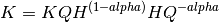
The Upper zone generates quick runoff $(Q_{q})$ using:

$Q_{q}=K*UZ^{(1+alpha)}$

here $K$ is the upper zone recession coefficient, and $\alpha$ determines the amount of non-linearity. Within HBV-96, the value of $K$ is determined from three other parameters: $\alpha$ , $KHQ$ , and $HQ$ (mm/day). The value of $HQ$ represents an outflow rate of the upper zone for which the recession rate is equal to $KHQ$ . if we define $UZ_{HQ}$ to be the content of the upper zone at outflow rate $HQ$ we can write the following equation:

$HQ=K*UZ_{HQ}^{(1+\alpha)}=KHQ*UZ_{HQ}$

If we eliminate $UZ_{HQ}$ we obtain:

$HQ=K*\left(\frac{HQ}{KHQ}\right)^{(1+\alpha)}$

Rewriting for $K$ results in:

$K=KQH^{(1-alpha)}HQ^{-alpha}$

Note

Note that the HBV-96 manual mentions that for a recession rate larger than 1 the timestap in the model will be adjusted.

The lower zone is a linear reservoir, which means the rate of slow runoff, $Q_{LZ}$ , which leaves this zone during one time step equals:

$Q_{LZ}=K_{LZ}*V_{LZ}$

where $K_{LZ}$ is the reservoir constant.

The upper zone is also a linear reservoir, but it is slightly more complicated than the lower zone because it is divided into two zones: A lower part in which interflow is generated and an upper part in which quick flow is generated (see Figure ref{fig:upper}).

Schematic view of the Upper zone

If the total water content of the upper zone, $V_{UZ}$ , is lower than a threshold $UZ1$ , the upper zone only generates interflow. On the other hand, if $V_{UZ}$ exceeds $UZ1$ , part of the upper zone water will runoff as quick flow:

$Q_{i} = K_{i}*min\{UZ1;V_{uz}\} Q_{q} = K_{q}*max\{(V_{UZ}-UZ1);0.0\}$

Where $Q_{i}$ is the amount of generated interflow in one time step, $Q_{q}$ is the amount of generated quick flow in one time step and $K_{i}$ and $K_{q}$ are reservoir constants for interflow and quick flow respectively.

The total runoff rate, $Q$ , is equal to the sum of the three different runoff components:

$Q=Q_{LZ}+Q_{i}+Q_{q}$

The runoff behaviour in the runoff response routine is controlled by two threshold values $P_{m}$ and $UZ1$ in combination with three reservoir parameters, $K_{LZ}$ , $K_{i}$ and $K_{q}$ . In order to represent the differences in delay times between the three runoff components, the reservoir constants have to meet the following requirement:

$K_{LZ}<K_{i}<K_{q}$

Description of the python module¶

Run the wflow_hbv hydrological model..

usage: wflow_hbv:

[-h][-v level][-F runinfofile][-L logfile][-C casename][-R runId]
[-c configfile][-T timesteps][-s seconds][-W][-E][-N][-U discharge]
[-P parameter multiplication][-X][-l loglevel]

-F: if set wflow is expected to be run by FEWS. It will determine: the timesteps from the runinfo.xml file and save the output initial conditions to an alternate location. Also set fewsrun=1 in the .ini file!

-f: Force overwrite of existing results

-T: Set the number of timesteps to run

-N: No lateral flow, use runoff response function to generate fast runoff

-s: Set the model timesteps in seconds

-I: re-initialize the initial model conditions with default

-i: Set input table directory (default is intbl)

-x: run for subcatchment only (e.g. -x 1)

-C: set the name of the case (directory) to run

-R: set the name runId within the current case

-L: set the logfile

-c: name of wflow the configuration file (default: Casename/wflow_hbv.ini).

-h: print usage information

-U: The argument to this option should be a .tss file with measured discharge in: [m^3/s] which the progam will use to update the internal state to match the measured flow. The number of columns in this file should match the number of gauges in the wflow_gauges.map file.
-u: list of gauges/columns to use in update. Format:: -u [1 , 4 ,13] The above example uses column 1, 4 and 13
-P: set parameter multiply dictionary (e.g: -P {‘self.FirstZoneDepth’ : 1.2}: to increase self.FirstZoneDepth by 20%, multiply with 1.2)
-p: set input parameter (dynamic, e.g. precip) multiply dictionary: (e.g: -p {‘self.Precipitation’ : 1.2} to increase Precipitation by 20%, multiply with 1.2)

-l: loglevel (most be one of DEBUG, WARNING, ERROR)

-X overwrites the initial values at the end of each timestep

$Author: schelle $ $Id: wflow_hbv.py 904 2014-01-13 14:39:24Z schelle $ $Rev: 904 $

class wflow_hbv.WflowModel(cloneMap, Dir, RunDir, configfile)¶

The user defined model class. All maps are defined here for documentation purposes

dynamic()¶

Below a list of variables that can be save to disk as maps or as timeseries (see ini file for syntax):

Dynamic variables

Variables:

self.SurfaceRunoff – Surface runoff in the kinematic wave [m^3/s]
self.WaterLevel – Water level in the kinematic wave [m] (above the bottom)
self.InterceptionStorage – actual interception storage [mm]
self.Snow – Snow depth [mm]
self.SnowWater – water content of the snow [mm]
self.LowerZoneStorage – water content of the lower zone [mm]
self.UpperZoneStorage – water content of the Upper zone [mm]
self.BaseFlow – Specific runoff (baseflow part) per cell [mm]
self.Percolation – actual percolation to the lower zone [mm]
self.SoilMoisture – actual soil moisture [mm]
self.QuickFlow – specific runoff (quickflow part) [mm]
self.RealQuickFlow – specific runoff (quickflow), If K upper zone is precalculated [mm]
self.CapFlux – capilary rise [mm]
self.SurfaceRunoffMM – Surfacerunoff in mm
self.KinWaveVolume – Volume in the kinematic wave reservoir

Static variables

Variables:	self.Altitude – The altitude of each cell [m] self.Bw – Width of the river [m] self.River – booolean map indicating the presence of a river [-] self.DLC – length of the river within a cell [m] self.ToCubic – Mutiplier to convert mm to m^3/s for fluxes

initial()¶

Initial part of the model, executed only once. Reads all static model information (parameters) and sets-up the variables used in modelling.

HBV Soil

Variables:	FC.tbl – Field Capacity (260.0) [mm] BetaSeepage.tbl – exponent in soil runoff generation equation (1.8) [-] LP.tbl – fraction of Fieldcapacity below which actual evaporation=potential evaporation (0.53000) K4.tbl – Recession constant baseflow (0.02307)

If SetKquickFlow is set to 1

Variables:	KQuickFlow.tbl – (0.09880) SUZ.tbl – Level over wich K0 is used (100.0) K0.tbl – (0.3)

If SetKquickFlow is set to 0

Variables:

KHQ.tbl – recession rate at flow HQ (0.09880)
HQ.tbl – high flow rate HQ for which recession rate of upper reservoir is known (3.27000)
AlphaNL.tbl – measure of non-linearity of upper reservoir (1.1)
PERC.tbl – Percolation from Upper to Lowerzone (0.4000) [mm/day]
CFR.tbl – Refreezing efficiency constant in refreezing of freewater in snow (0.05000)
Pcorr.tbl – Correction factor for precipitation (1.0)
RFCF.tbl – Correction factor for rainfall (1.0)
SFCF.tbl – Correction factor for snowfall(1.0)
Cflux.tbl – Maximum capillary rise from runoff response routine to soil moisture routine (2.0)
ICF.tbl – Maximum interception storage (in forested AND non-forested areas) (2.0)
CEVPF.tbl – Correction factor for potential evaporation (1.0)
EPF.tbl – Exponent of correction factor for evaporation on days with precipitation(0.0)
ECORR.tbl – Evap correction (1.0)

Snow modelling parameters

Variables:	TTI.tbl – critical temperature for snowmelt and refreezing (1.000) [oC] TT.tbl – defines interval in which precipitation falls as rainfall and snowfall (-1.41934) [oC] Cfmax.tbl – meltconstant in temperature-index ( 3.75653) [-] WHC.tbl – fraction of Snowvolume that can store water (0.1) [-]

resume()¶: read initial state maps (they are output of a previous call to suspend())

stateVariables()¶

returns a list of state variables that are essential to the model. This list is essential for the resume and suspend functions to work.

This function is specific for each model and must be present.

Variables:

self.SurfaceRunoff – Surface runoff in the kin-wave resrvoir [m^3/s]
self.WaterLevel – Water level in the kin-wave resrvoir [m]
self.DrySnow – Snow pack [mm]
self.FreeWater – Available free water [mm]
self.UpperZoneStorage – Water in the upper zone [mm]
self.LowerZoneStorage – Water in the lower zone [mm]
self.SoilMoisture – Soil moisture [mm]
self.InterceptionStorage – Amount of water on the Canopy [mm]

supplyCurrentTime()¶

gets the current time in seconds after the start of the run

Ouput:

time in seconds since the start of the model run

suspend()¶: Suspends the model to disk. All variables needed to restart the model are saved to disk as pcraster maps. Use resume() to re-read them

updateRunOff()¶: Updates the kinematic wave reservoir

wflow_hbv.main(argv=None)¶: Perform command line execution of the model.

wflow_hbv.multdynapars = {}¶: Dictionary with parameters and multipliers (dynamic) (used in calibration)

wflow_hbv.multpars = {}¶: Dictionary with parameters and multipliers (static) (used in calibration)

wflow_hbv.updateCols = []¶: Column sused in updating

wflow_hbv.usage(*args)¶

Print usage information

*args: command line arguments given

wflow_hbv.wflowVersion = '$Revision: 904 $ $Date: 2014-01-13 15:39:24 +0100 (Mon, 13 Jan 2014) $'¶: revision of the model