The wflow_sbm Model¶

Introduction¶

The soil part of wflow_sbm model follows the same concepts as the topog_sbm model. topog_sbm is specifically designed to similate fast runoff processes in small catchments while wflow_sbm can be applied more widely. The main differences are:

The addition of evapotranspiration losses
The addition of a percolary rise
Wflow routes water over a D8 network while topog uses an element network based on contour lines and trajectories.
The (optional) addition of sub-cell runoff to be able to run on larger grid sizes

The sections below describe the working of the model in more detail.

The rainfall interception model¶

The analytical (Gash) model¶

The analytical model of rainfall interception is based on Rutter’s numerical model . The simplifications that introduced allow the model to be applied on a daily basis, although a storm-based approach will yield better results in situations with more than one storm per day . The amount of water needed to completely saturate the canopy is defined as:

$P'=\frac{-\overline{R}S}{\overline{E}_{w}}ln\left[1-\frac{\overline{E}_{w}}{\overline{R}}(1-p-p_{t})^{-1}\right]$

where $\overline{R}$ is the average precipitation intensity on a saturated canopy and $\overline{E}_{w}$ the average evaporation from the wet canopy and with the vegetation parameters $S$ , $p$ and $p_t$ as defined previously. The model uses a series of expressions to calculate the interception loss during different phases of a storm. An analytical integration of the total evaporation and rainfall under saturated canopy conditions is then done for each storm to determine average values of $\overline{E}_{w}$ and $\overline{R}$ . The total evaporation from the canopy ( the total interception loss) is calculated as the sum of the components listed in the table below. Interception losses from the stems are calculated for days with $P\geq S_{t}/p_{t}$ . $p_t$ and $S_t$ are small and neglected in the wflow_sbm model.

Table: Formulation of the components of interception loss according to Gash:

For $m$ small storms ( $P_{g}<{P'}_{g}$ )	$(1-p-p_{t})\sum_{j=1}^{m}P_{g,j}$
Wetting up the canopy in $n$ large storms ( $P_{g}\geq{P'}_{g}$ )	$n(1-p-p_{t}){P'}_{g}-nS$
Evaporation from saturated canopy during rainfall	$\overline{E}/\overline{R}\sum_{j=1}^{n}(P_{g,j}-{P'}_{g})$
Evaporation after rainfall ceases for $n$ large storms	$nS$
Evaporation from trunks in $q$ storms that fill the trunk storage	$qS_{t}$
Evaporation from trunks in ( $m+n-q$ ) storms that do not fill the trunk storage	$p_{t}\sum_{j=1}^{m+n-q}P_{g,j}$

In applying the analytical model, saturated conditions are assumed to occur when the hourly rainfall exceeds a certain threshold. Often a threshold of 0.5 mm/hr is used . $\overline{R}$ is calculated for all hours when the rainfall exceeds the threshold to give an estimate of the mean rainfall rate onto a saturated canopy.

Gash (1979) has shown that in a regression of interception loss on rainfall (on a storm basis) the regression coefficient should equal to $\overline{E}_w/\overline{R}$ . Assuming that neither $\overline{E}_w$ nor $\overline{R}$ vary considerably in time, $\overline{E}_w$ can be estimated in this way from $\overline{R}$ in the absence of above-canopy climatic observations . Values derived in this way generally tend to be (much) higher than those calculated with the penman-montieth equation .

The modified rutter model¶

For subdaily timesteps the model uses a simplification of the Rutter model. The simplyfied model is solved explicitly and does not take drainage from the canopy into account.

def rainfall_interception_modrut(Precipitation,PotEvap,CanopyStorage,CanopyGapFraction,Cmax):
   """
   Interception according to a modified Rutter model. The model is solved
   explicitly and there is no drainage below Cmax.

   Returns:
       - NetInterception: P - TF - SF (may be different from the actual wet canopy evaporation)
       - ThroughFall:
       - StemFlow:
       - LeftOver: Amount of potential eveporation not used
       - Interception: Actual wet canopy evaporation in this thimestep
       - CanopyStorage: Canopy storage at the end of the timestep

   """

   ##########################################################################
   # Interception according to a modified Rutter model with hourly timesteps#
   ##########################################################################

   p = CanopyGapFraction
   pt = 0.1 * p

   # Amount of P that falls on the canopy
   Pfrac = (1 - p -pt) * Precipitation

   # S cannot be larger than Cmax, no gravity drainage below that
   DD = ifthenelse (CanopyStorage > Cmax , Cmax - CanopyStorage , 0.0)
   self.CanopyStorage = CanopyStorage - DD

   # Add the precipitation that falls on the canopy to the store
   CanopyStorage = CanopyStorage + Pfrac

   # Now do the Evap, make sure the store does not get negative
   dC = -1 * min(CanopyStorage, PotEvap)
   CanopyStorage = CanopyStorage + dC

   LeftOver = PotEvap +dC; # Amount of evap not used


   # Now drain the canopy storage again if needed...
   D = ifthenelse (CanopyStorage > Cmax , CanopyStorage - Cmax , 0.0)
   CanopyStorage = CanopyStorage - D

   # Calculate throughfall
   ThroughFall = DD + D + p * Precipitation
   StemFlow = Precipitation * pt

   # Calculate interception, this is NET Interception
   NetInterception = Precipitation - ThroughFall - StemFlow
   Interception = -dC

   return NetInterception, ThroughFall, StemFlow, LeftOver, Interception, CanopyStorage

The soil model¶

Infiltration¶

If the surface is (partly) saturated the rainfall that falls onto the saturated area is added to the surface runoff component. Infiltration of the remaining water is determined as follows:

First the soil infiltration capacity is adjusted in case the soil is frozen. The remaining storage capacity of the unsaturated store is determined. The infiltrating water is split is two parts, the part that fall on compacted areas and the part that fall on non-compacted areas. First the amount of water that infiltrates in non-compacted areas is calculated by taking the mimimum of the remaining storage capacity, the maximum soil infiltration rate and the water on non-compated areas. After adding the infiltrated water to the unsaturated store the same is done for the compated areas after updatting the remaining storage capacity.

The wflow_sbm soil water accounting scheme¶

A detailed description of the SBM model has been given by [vertessy]. Briefly: the soil is considered as a bucket with a certain depth ( $z_{t}$ ), divided into a saturated store ( $S$ ) and an unsaturated store ( $U$ ), the magnitudes of which are expressed in units of depth. The top of the $S$ store forms a pseudo-water table at depth $z_{i}$ such that the value of $S$ at any time is given by:

$S=(z_{t}-z_{i})(\theta_{s}-\theta_{r})$

where:

$\theta_{s}$ and $\theta_{r}$ are the saturated and residual soil water contents, respectively.

The unsaturated store ( $U$ ) is subdivided into storage ( $U_{s}$ ) and deficit ( $U_{d}$ ) which are again expressed in units of depth:

$U_{d}=(\theta_{s}-\theta_{r})z_{i}-U U_{s}=U-U_{d}$

The saturation deficit ( $S_{d}$ ) for the soil profile as a whole is defined as:

$S_{d}=(\theta_{s}-\theta_{r})z_{t}-S$

All infiltrating rainfall enters the $U$ store first. The transfer of water from the $U$ store to the $S$ store ( $st$ ) is controlled by the saturated hydraulic conductivity {} at depth $z_{i}$ and the ratio between $U$ and $S_{d}$ :

$st=K_{\mathit{sat}}\frac{U_{s}}{S_{d}}$

Hence, as the saturation deficit becomes smaller, the rate of the transfer between the $U$ and $S$ stores increases.

Schematisation of the soil within the wflow_sbm model

Saturated conductivity ( $K_{sat}$ ) declines with soil depth ( $z$ ) in the model according to:

where:

$K_{0}$ is the saturated conductivity at the soil surface and

$f$ is a scaling parameter [ $m^{-1}$ ]

The scaling parameter $f$ is defined by:

$f=\frac{\theta_{s}-\theta_{r}}{M}$

with $\theta_{s}$ and $\theta_{r}$ as defined previously and $M$ representing a model parameter (expressed in meters).

Figure: Plot of the relation between depth and conductivity for different values of M

(Source code, png, hires.png, pdf)

The $S$ store can be drained laterally via subsurface flow according to:

$sf=K_{0}\mathit{tan}(\beta)e^{-S_{d}/M}$

where:

$\beta$ is element slope angle [deg.]

$sf$ is the calculated subsurface flow [ $m^{2}d^{-1}$ ]

$S_{d}$ is the saturation deficit defined as: ( $(\theta_{s}-\theta_{r})z_{t}-S$ )

with $M$ and $S_{d}$ as defined previously. A schematic representation of the various hydrological processes and pathways modelled by SBM (infiltration, exfiltration, Hortonian and saturation overland flow, subsurface flow) is provided by verstessy (1999).

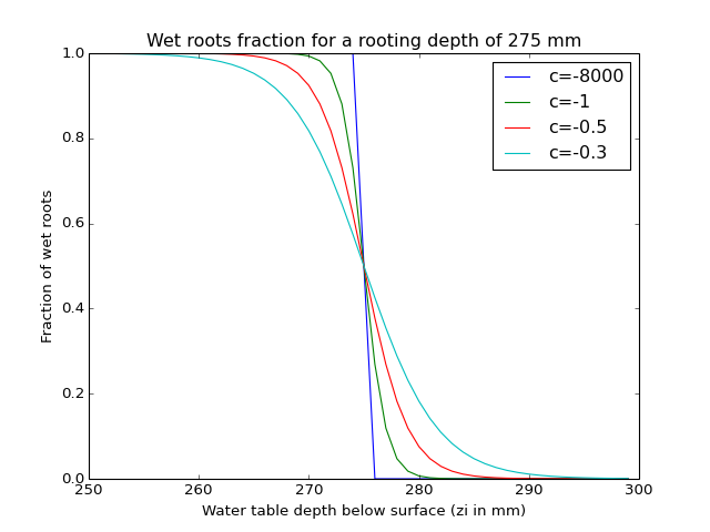
The original SBM model does not include transpiration or a notion of capilary rise. In wflow_sbm transpiration is first taken from the $S$ store if the roots reach the water table $z_{i}$ . If the $S$ store cannot satisfy the demand the $U$ store is used next. First the number of wet roots is determined (going from 1 to 0) using an sigmoid function as follows:

$WetRoots = 1.0/(1.0 + e^{-SharpNess (WaterTable - RootingDepth)})$

Here the sharpness parameter (by default a large negative value, -80000.0) parameter determines if there is a stepwise output or a more gradual output (default is stepwise). WaterTable is the level of the Water table in the gridcell in mm below the surface, RootingDepth is the maximum depth of the roots also in mm below the surface. For all values of WaterTable smaller that RootingDepth a value of 1 is returned if they are equal a value of 0.5 is returned if the WaterTable is larger than the RootingDepth a value of 0 is returned. The returned WetRoots fraction is multiplied by the potential evaporation (and limited by the available water in saturated zone) to get the transpiration from the saturated part of the soil.

Figure: Plot showing the fraction of wet roots for different values of c for a RootingDepth of 275mm

(Source code, png, hires.png, pdf)

Next the remaining potential evaporation is used to extract water from the unsaturated store:

FirstZoneDepth = FirstZoneDepth - ActEvapSat
RestPotEvap = PotTrans - ActEvapSat

# now try unsat store
AvailCap = min(1.0,max (0.0,(WTable - RootingDepth)/(RootingDepth + 1.0)))

MaxExtr = AvailCap  * UStoreDepth
ActEvapUStore = min(MaxExtr,RestPotEvap,UStoreDepth)
UStoreDepth = UStoreDepth - ActEvapUStore

ActEvap = ActEvapSat + ActEvapUStore

Capilary rise is determined using the following approach: first the $K_{sat}$ is determined at the water table $z_{i}$ ; next a potential capilary rise is determined from the minimum of the $K_{sat}$ , the actual transpiration taken from the $U$ store, the available water in the $S$ store and the deficit of the $U$ store. Finally the potential rise is scaled using the distance between the roots and the water table using:

$CS=CSF/(CSF+z_{i}-RT)$

in which $CS$ is the scaling factor to multiply the potential rise with, $CSF$ is a model parameter (default = 100, use CapScale.tbl to set differently) and $RT$ the rooting depth. If the roots reach the water table ( $RT>z_{i}$ ) $CS$ is set to zero thus setting the capilary rise to zero.

Water in the saturated store is transferred laterally along the DEM using the following steps:
1. a maximum flux for each cell is determined by determining the {} over the saturated part and the available water in each cell
2. water is routed downslope (using the PCRaster accucapacityflux operator) by multiplying the {} by the slope and limiting the flux the the maximum determined in the previous step
3. the program can either use the DEM to route the water or (more appropriate in flat areas) the actual slope of the water table. The latter option slows down the program considerably
surplus water in cells as a result of the previous step is added to the kinematic wave reservoir

Soil temperature¶

The near surface soil temperature is modelled using a simple equation [Wigmosta]:

$T_s^{t} = T_s^{t-1} + w (T_a - T_s^{t-1})$

where $T_s^{t}$ is the near-surface soil temperature at time t, $T_a$ is air temperature and $w$ is a weighting coefficient determined through calibration (default is 0.1125 for daily timesteps, 0.9 for 3-hourly timesteps)

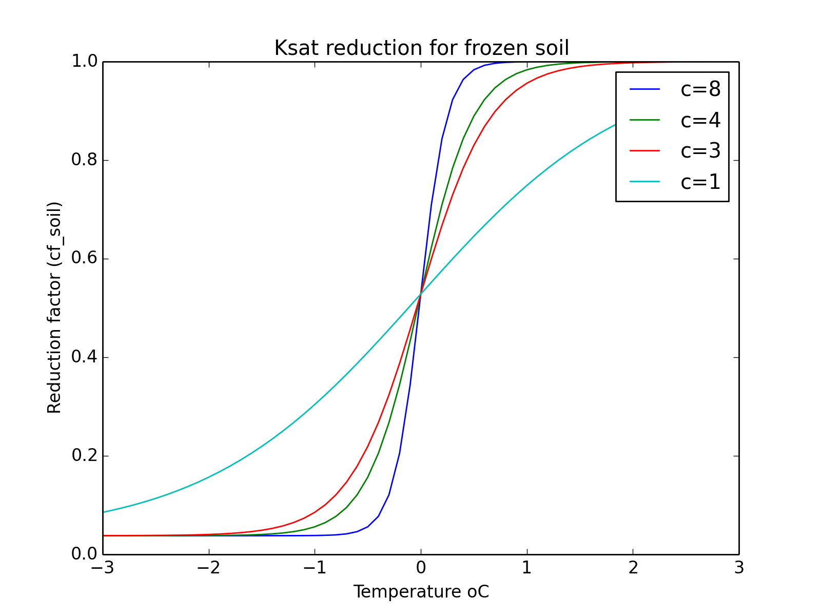
if T_s < 0 than a K_{sat} reduction factor (default 0.038) is applied. An S-curve (see plot below) is used to make a smooth transition (a c-factor of 8 is used).

(Source code, png, hires.png, pdf)

Sub-grid runoff generation¶

Sub-grid runoff generaten can be switched on on off in the configuration file. In general this feature is used if the grid cell size is relatively lager compared to the variation of topography. In addition you will need to have information on the ditribution of altotude within a grid-cell. Depending on the topography sub-grid runoff generation may be useful aroun 1x1km and larger.

The basis is formed by a sigmoid ( $S$ ) function that is fitted using a 10, 50 and 90 percentile DEM. The $S$ function is defined as:

$S = 1.0/(b + e^{(-c (X - a))})$

Where:

X = input variable (in this case the absolute scaled groundwater level)

b = 1.0

c = sharpness parameter. Higher values give sharper step

a = centre-point of the curve (normally the 50% DEM)

The $c$ parameter is estimated by reversing the function above to:

$c = log(1.0/p - 1)/(dem_{p} - dem_{50})$

where:

percentile is the percentile of $dem_{p}$

$dem_{50}$ is the average altitude in the gridcell

$dem_{p}$ is the altitude below with percentile (p) cells of the dem are found

The outcome of the $S$ will range from 0 to 1 for inputs ranging from the minimum altitude to the maximum altitude (within the gridcell). Thereore, the calculated groundwater levels within the cell are scale to match the minimum and maximum altitude within the cell using:

$G_s = (A_{max}-A_{min})/FZT/GWPerc$

where:

$G_s$ is the scaling factor

$A_{max}$ the maximum altitude within the cell

$A_{min}$ the minumum altitude within the cell

$FZT$ the total thickness of the soil in the model

$GWperc$ is a dimensionless parameter (from >0 to 1) that determines which part of the soil profile generates runoff. If it is 1 runoff is generated whenever there is groundwater in the system. If it is 0.1 only the top 10 % of the soil profile generated runoff

self.DemMax=readmap(self.Dir + "/staticmaps/wflow_demmax")
self.DrainageBase=readmap(self.Dir + "/staticmaps/wflow_demmin")
self.CC = min(100.0,-log(1.0/0.1 - 1)/min(-0.1,self.DrainageBase - self.Altitude))
self.GWScale = (self.DemMax-self.DrainageBase)/self.FirstZoneThickness / self.RunoffGeneratingGWPerc

Note

at present the model uses the drainage base (minimum DEM) and treats this as the 10% percentile to which the curve is fitted. So at present only two points are used (10 % and 50%)

Warning

This is an poorly tested feature

In the dynamic section of the model the absolute groundwater level is determined and scaled before it is fed into the $S$ curve function. The result is a estimated saturated fraction within a the gridcell. The saturated fraction is used to generated Saturation Overland Flow (SOF) and generate ouflow from the groundwater reservoir:

The saturated conductivity for the average groundwaterlevel is determined
The available water at the surface is multiplied by the saturated fraction and added to the kinematic wave reservoir (SOF)
Outflow from the groundwater reservoir is determined using average slope multiplied by the conductivity and the saturated fraction limited by the amount of water in the groundwater reservoir.

in dynamic:

self.AbsoluteGW=self.DemMax-(self.zi*self.GWScale)
self.SubCellFrac = sCurve(self.AbsoluteGW,c=self.CC,a=self.Altitude+1.0)
self.SubCellRunoff = self.SubCellFrac * FreeWaterDepth
self.SubCellGWRunoff = min(self.SubCellFrac * self.FirstZoneDepth,\
    self.SubCellFrac * self.Slope * self.FirstZoneKsatVer * \
    exp(-self.f * self.zi) * self.timestepsecs/self.basetimestep)
self.FirstZoneDepth=self.FirstZoneDepth-self.SubCellGWRunoff
FreeWaterDepth = FreeWaterDepth - self.SubCellRunoff

Kinematic wave and River Width¶

The river width is determined from the DEM the upstream area and yearly average discharge ([Finnegan]):

The early average Q at outlet is scaled for each point in the drainage network with the upstream area. $\alpha$ ranges from 5 to > 60. Here 5 is used for hardrock, largre values are used for sediments

Implementation:

upstr = catchmenttotal(1, self.TopoLdd)
Qscale = upstr/mapmaximum(upstr) * Qmax
W = (alf * (alf + 2.0)**(0.6666666667))**(0.375) * Qscale**(0.375) *\
     (max(0.0001,windowaverage(self.Slope,celllength() * 4.0)))**(-0.1875) *\
     self.N **(0.375)
RiverWidth = W

The table below list commonly used Manning’s N values (in the N_River .tbl file). Please note that the values for non river cells may arguably be set significantly higher. (Use N.tbl for non-river cells and N_River.tbl for river cells)

Manning’s N values
Type of Channel and Description	Minimum	Normal	Maximum
Main Channels
clean, straight, full stage, no rifts or deep pools	0.025	0.03	0.033
same as above, but more stones and weeds	0.03	0.035	0.04
clean, winding, some pools and shoals	0.033	0.04	0.045
same as above, but some weeds and stones	0.035	0.045	0.05
same as above, lower stages, more ineffective slopes and sections	0.04	0.048	0.055
same as second with more stones	0.045	0.05	0.06
sluggish reaches, weedy, deep pools	0.05	0.07	0.08
very weedy reaches, deep pools, or floodways with heavy stand of timber and underbrush	0.075	0.1	0.15
Mountain streams
bottom: gravels, cobbles, and few boulders	0.03	0.04	0.05
bottom: cobbles with large boulders	0.04	0.05	0.07

Dynamic wave¶

Warning

As of version 0.93 this is moved to the wflow_wave module.

An experimental implementation of the full dynamic wave equations has been implemented. The current implementation is fairly unstable and very slow. It can be switched on by setting dynamicwave=1 in the [dynamicwave] section of the ini file. See below for an example:

[dynamicwave]
# Switch on dynamic wave for main rivers
dynamicwave=1

# Number of timeslices per dynamic wave substep
TsliceDyn=100

# number of substeps for the dynamic wave with respect to the model timesteps
dynsubsteps=24

# map with level boundary points
wflow_hboun = staticmaps/wflow_outlet.map

# Optional river map for the dynamic wave that must be the same size or smaller as that of the
# kinematic wave
wflow_dynriver = staticmaps/wflow_dynriver.map

# a fixed water level for each non-zero point in the wflow_hboun map
# level > 0.0 use that level
# level == 0.0 use supplied timeseries (see levelTss)
# level < 0.0 use upstream water level
fixedLevel = 3.0

# if this is set the program will try to keep the volume at the pits at
# a constant value
lowerflowbound = 1

# instead of a fixed level a tss file with levels for each timesteps and each
# non-zero value in the wflow_hboun map
#levelTss=intss/Hboun.tss

# If set to 1 the program will try to optimise the timestep
# Experimental, mintimestep is the smallest to be used
#AdaptiveTimeStepping = 1
#mintimestep =1.0

A description of the implementation of the dynamicwave is given on the pcraster website.

In addition to the settings in the ini file you need to give the model additional maps or lookuptables:

ChannelDepth.[map|tbl] - depth of the main channel in metres
ChannelRoughness.[map|tbl] - manning roughness coefficient (default = 0.03)
ChannelForm.[map|tbl] - form of the chnaggel (default = 0.0)
FloodplainWidth.[map|tbl] - width of the floodplain in metres (default = )

The following variables for the dynamicwave function are set as follows:

ChannelBottomLevel - Taken from the dem
ChannelLength - Taken from the length in the kinematic wave
ChannelBottomWidth - taken from the wflow_riverwidth map (this map can be user supplied or when it is not supplied a geomorphological relation is used)

Becuase the dynamic wave can be unstable priming the model with new initial conditions is best done in several steps:

Run the model with the -I option and the dynamic wave switch off
Copy back the resulting state files to the instate directory
Re-run the model with the without the -I option
Copy back the resulting states of the Dynamic wave to the instate directory

Model variables stores and fluxes¶

The diagram below shows the stores and fluxes in the model in terms of internal variable names. It onlys shows the soil and Kinematic wave reservoir, not the canopy model.

$digraph grids { compound=true; node[shape=record]; UStoreDepth [shape=box]; OutSide [style=dotted]; FirstZoneDepth [shape=box]; UStoreDepth -> FirstZoneDepth [label="Transfer [mm]"]; FirstZoneDepth -> UStoreDepth [label="CapFlux [mm]"]; FirstZoneDepth ->KinematicWaveStore [label="ExfiltWaterCubic [m^3/s]"]; "OutSide" -> UStoreDepth [label="ActInfilt [mm]"]; UStoreDepth -> OutSide [label="ActEvapUStore [mm]"]; FirstZoneDepth -> OutSide [label="ActEvap-ActEvapUStore [mm]"]; FirstZoneDepth -> KinematicWaveStore [label="SubCellGWRunoffCubic [m^3/s]"]; "OutSide" -> KinematicWaveStore [label="SubCellRunoffCubic [m^3/s]"]; "OutSide" -> KinematicWaveStore [label="RunoffOpenWater [m^3/s]"] ; "OutSide" -> KinematicWaveStore [label="FreeWaterDepthCubic [m^3/s]"] ; }$

Processing of meteorological forcing data¶

Although the model has been setup to do as little data processing as possible it includes an option to apply an altitude correction to the temperature inputs. The three squares below demonstrate the principle.

digraph grids {
node[shape=record];
a[label="{5|5|5}|{5|5|5}|{5|5|5}"];
b[label="{1|2|3}|{4|5|6}|{7|8|9}"];
c[label="{4|3|2}|{1|0|-1}|{-2|-3|-4}"];
"Average T input grid" -> a
"Correction per cell" -> b
"Resulting T" -> c
}

wflow_sbm takes the correction grid as input and applies this to the input temperature. The correction grid has to be made outside of the model. The correction grid is optional.

Note

The temperature correction map is specified in the model section of the ini file:

[model] TemperatureCorrectionMap=NameOfTheMap

If the entry is not in the file the correction will not be applied

Guidelines for wflowsbm model parameters¶

The tables below shows the most important parameters and suggested ranges

CanopyGapFraction file:///media/schelle/BIG/LINUX/wflow/cases/maas/intbl/Cfmax.tbl

EoverR - Ratio of average wet canopy evaporation rate over precipitation rate - usually between 0.06 and 0.15 depending on climate and site.
FirstZoneCapacity -

FirstZoneKsatVer.tbl
file:///media/schelle/BIG/LINUX/wflow/cases/maas/intbl/FirstZoneMinCapacity.tbl
file:///media/schelle/BIG/LINUX/wflow/cases/maas/intbl/InfiltCapPath.tbl
file:///media/schelle/BIG/LINUX/wflow/cases/maas/intbl/InfiltCapSoil.tbl
file:///media/schelle/BIG/LINUX/wflow/cases/maas/intbl/M.tbl
file:///media/schelle/BIG/LINUX/wflow/cases/maas/intbl/MaxCanopyStorage.tbl
file:///media/schelle/BIG/LINUX/wflow/cases/maas/intbl/MaxLeakage.tbl
file:///media/schelle/BIG/LINUX/wflow/cases/maas/intbl/N_River.tbl
file:///media/schelle/BIG/LINUX/wflow/cases/maas/intbl/N.tbl
file:///media/schelle/BIG/LINUX/wflow/cases/maas/intbl/RootingDepth.tbl
file:///media/schelle/BIG/LINUX/wflow/cases/maas/intbl/RunoffGeneratingGWPerc.tbl
file:///media/schelle/BIG/LINUX/wflow/cases/maas/intbl/thetaR.tbl
file:///media/schelle/BIG/LINUX/wflow/cases/maas/intbl/thetaS.tbl
file:///media/schelle/BIG/LINUX/wflow/cases/maas/intbl/TT.tbl
file:///media/schelle/BIG/LINUX/wflow/cases/maas/intbl/TTI.tbl
file:///media/schelle/BIG/LINUX/wflow/cases/maas/intbl/WHC.tbl

References¶

[vertessy]

Vertessy, R.A. and H. Elsenbeer, “Distributed modelling of storm flow generation in an Amazonian rainforest catchment: effects of model parameterization,” Water Resources Research, vol. 35, no. 7, pp. 2173–2187, 1999.

[Finnegan]

Noah J. Finnegan et al 2005 Controls on the channel width of rivers: Implications for modeling fluvial incision of bedrock”

[Wigmosta]

Wigmosta, M. S., L. J. Lane, J. D. Tagestad, and A. M. Coleman (2009), Hydrologic and erosion models to assess land use and management practices affecting soil erosion, Journal of Hydrologic Engineering, 14(1), 27-41.

wflow_sbm module documentation¶

Run the wflow_sbm hydrological model..

usage

wflow_sbm [-h][-v level][-F runinfofile][-L logfile][-C casename][-R runId]
      [-c configfile][-T last_step][-S first_step][-s seconds][-W][-E][-N][-U discharge]
      [-P parameter multiplication][-X][-f][-I][-i tbl_dir][-x subcatchId][-u updatecols]
      [-p inputparameter multiplication][-l loglevel]
      
-F: if set wflow is expected to be run by FEWS. It will determine
    the timesteps from the runinfo.xml file and save the output initial
    conditions to an alternate location. Also set fewsrun=1 in the .ini file!
    
-X: save state at the end of the run over the initial conditions at the start        

-f: Force overwrite of existing results    

-T: Set last timestep

-S: Set the start timestep (default = 1)

-s: Set the model timesteps in seconds

-I: re-initialize the initial model conditions with default

-i: Set input table directory (default is intbl)

-x: Apply multipliers (-P/-p ) for subcatchment only (e.g. -x 1)

-C: set the name  of the case (directory) to run

-R: set the name runId within the current case

-L: set the logfile

-E: Switch on reinfiltration of overland flow

-c: name of wflow the configuration file (default: Casename/wflow_sbm.ini). 

-h: print usage information

-W: If set, this flag indicates that an ldd is created for the water level
    for each timestep. If not the water is assumed to flow according to the 
    DEM. Wflow will run a lot slower with this option. Most of the time
    (shallow soil, steep topography) you do not need this option. Also, if you 
    need it you migth actually need another model.
    
-U: The argument to this option should be a .tss file with measured discharge in
    [m^3/s] which the progam will use to update the internal state to match 
    the measured flow. The number of columns in this file should match the 
    number of gauges in the wflow\_gauges.map file.

-u: list of gauges/columns to use in update. Format:
    -u [1 , 4 ,13]
    The above example uses column 1, 4 and 13
    
-P: set parameter multiply dictionary (e.g: -P {'self.FirstZoneDepth' : 1.2}
    to increase self.FirstZoneDepth by 20%, multiply with 1.2)
    
-p: set input parameter (dynamic, e.g. precip) multiply dictionary 
    (e.g: -p {'self.Precipitation' : 1.2} to increase Precipitation 
    by 20%, multiply with 1.2)    
    
-l: loglevel (most be one of DEBUG, WARNING, ERROR)

$Author: schelle $ $Id: wflow_sbm.py 900 2014-01-09 17:41:06Z schelle $ $Rev: 900 $

wflow_sbm.SnowPackHBV(Snow, SnowWater, Precipitation, Temperature, TTI, TT, Cfmax, WHC)¶

HBV Type snowpack modelling using a Temperature degree factor. All correction factors (RFCF and SFCF) are set to 1. The refreezing efficiency factor is set to 0.05.

Variables:	Snow – SnowWater – Precipitation – Temperature –
Returns:	Snow,SnowMelt,Precipitation

class wflow_sbm.WflowModel(cloneMap, Dir, RunDir, configfile)¶

Bases: pcraster.framework.dynamicPCRasterBase.DynamicModel

Changed in version 0.91: - Calculation of GWScale moved to resume() to allow fitting.

New in version 0.91: - added S-curve for freezing soil infiltration reduction calculations

dynamic()¶

Stuf that is done for each timestep

Below a list of variables that can be save to disk as maps or as timeseries (see ini file for syntax):

Dynamic variables

Variables:

self.Precipitation – Gross precipitation [mm]
self.Temperature – Air temperature [oC]
self.PotenEvap – Potential evapotranspiration [mm]
self.PotTrans – Potential Transpiration (after subtracting Interception from PotenEvap) [mm]
self.Interception – Actual rainfall interception [mm]
self.ActEvap – Actual evaporation [mm]
self.SurfaceRunoff – Surface runoff in the kinematic wave [m^3/s]
self.SurfaceRunoffDyn – Surface runoff in the dyn-wave resrvoir [m^3/s]
self.WaterLevelDyn – Water level in the dyn-wave resrvoir [m^]
self.ActEvap – Actual EvapoTranspiration [mm]
self.WaterLevel – Water level in the kinematic wave [m] (above the bottom)
self.ActInfilt – Actual infiltration into the unsaturated zone [mm]
self.CanopyStorage – actual canopystorage (only for subdaily timesteps) [mm]
self.FirstZoneDepth – Amount of water in the saturated store [mm]
self.UStoreDepth – Amount of water in the unsaturated store [mm]
self.Snow – Snow depth [mm]
self.SnowWater – water content of the snow [mm]
self.TSoil – Top soil temperature [oC]
self.FirstZoneDepth – amount of available water in the saturated part of the soil [mm]
self.UStoreDepth – amount of available water in the unsaturated zone [mm]
self.Transfer – downward flux from unsaturated to saturated zone [mm]
self.CapFlux – capilary flux from saturated to unsaturated zone [mm]
self.CanopyStorage – Amount of water on the Canopy [mm]

Static variables

Variables:	self.Altitude – The altitude of each cell [m] self.Bw – Width of the river [m] self.River – booolean map indicating the presence of a river [-] self.DLC – length of the river within a cell [m] self.ToCubic – Mutiplier to convert mm to m^3/s for fluxes

initial()¶

Initial part of the model, executed only once. Reads all static data from disk

Soil

Variables:

M.tbl – M parameter in the SBM model. Governs the decay of Ksat with depth [-]
thetaR.tbl – Residual water content [mm/mm]
thetaS.tbl – Saturated water content (porosity) [mm/mm]
FirstZoneKsatVer.tbl – Saturated conductivity [mm/d]
PathFrac.tbl – Fraction of compacted area per grid cell [-]
InfiltCapSoil.tbl – Soil infiltration capacity [m/d]
InfiltCapPath.tbl – Infiltration capacity of the compacted areas [mm/d]
FirstZoneMinCapacity.tbl – Minimum wdepth of the soil [mm]
FirstZoneCapacity.tbl – Maximum depth of the soil [m]
RootingDepth.tbl – Depth of the roots [mm]
MaxLeakage.tbl – Maximum leakage out of the soil profile [mm/d]
CapScale.tbl – Scaling factor in the Capilary rise calculations (100) [mm/d]
RunoffGeneratingGWPerc – Fraction of the soil depth that contributes to subcell runoff (0.1) [-]
rootdistpar.tbl – Determine how roots are linked to water table. The number should be negative. A more negative number means that all roots are wet if the water table is above the lowest part of the roots. A less negative number smooths this. [mm] (default = -80000)

Canopy

Variables:	CanopyGapFraction.tbl – Fraction of precipitation that does not hit the canopy directly [-] MaxCanopyStorage.tbl – Canopy interception storage capacity [mm] EoverR.tbl – Ratio of average wet canopy evaporation rate over rainfall rate [-]

Surface water

Variables:	N.tbl – Manning’s N parameter N_river.tbl – Manning’s N parameter fro cells marked as river

Snow and frozen soil modelling parameters

Variables:

cf_soil.tbl – Soil infiltration reduction factor when soil is frozen [-] (< 1.0)
TTI.tbl – critical temperature for snowmelt and refreezing (1.000) [oC]
TT.tbl – defines interval in which precipitation falls as rainfall and snowfall (-1.41934) [oC]
Cfmax.tbl – meltconstant in temperature-index ( 3.75653) [-]
WHC.tbl – fraction of Snowvolume that can store water (0.1) [-]
w_soil.tbl – Soil temperature smooth factor. Given for daily timesteps. (0.1125) [-] Wigmosta, M. S., L. J. Lane, J. D. Tagestad, and A. M. Coleman (2009).

resume()¶

stateVariables()¶

returns a list of state variables that are essential to the model. This list is essential for the resume and suspend functions to work.

This function is specific for each model and must be present.

Variables:

self.SurfaceRunoff – Surface runoff in the kin-wave resrvoir [m^3/s]
self.SurfaceRunoffDyn – Surface runoff in the dyn-wave resrvoir [m^3/s]
self.WaterLevel – Water level in the kin-wave resrvoir [m]
self.WaterLevelDyn – Water level in the dyn-wave resrvoir [m^]
self.Snow – Snow pack [mm]
self.SnowWater – Snow pack water [mm]
self.TSoil – Top soil temperature [oC]
self.UStoreDepth – Water in the Unsaturated Store [mm]
self.FirstZoneDepth – Water in the saturated store [mm]
self.CanopyStorage – Amount of water on the Canopy [mm]

supplyCurrentTime()¶: gets the current time in seconds after the start of the run

suspend()¶

updateRunOff()¶: Updates the kinematic wave reservoir. Should be run after updates to Q

wflow_sbm.actEvap_SBM(RootingDepth, WTable, UStoreDepth, FirstZoneDepth, PotTrans, smoothpar)¶

Actual evaporation function:

first try to get demand from the saturated zone, using the rootingdepth as a limiting factor
secondly try to get the remaining water from the unsaturated store
it uses an S-Curve the make sure roots het wet/dry gradually (basically) representing a root-depth distribution

Input:

RootingDepth,WTable, UStoreDepth,FirstZoneDepth, PotTrans, smoothpar

Output:

ActEvap, FirstZoneDepth, UStoreDepth ActEvapUStore

wflow_sbm.main(argv=None)¶: Perform command line execution of the model.

wflow_sbm.usage(*args)¶